G-DIRT
Germplasm Duplicate Identification and Removal Tool

G-DIRT Help for executing the tool and understanding the results

Input file preparation
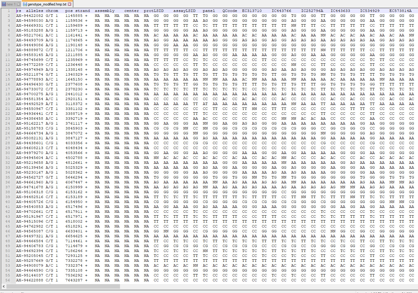
The input file to GDIRT server has to be given in hapmap format, where markers are represented in rows and genotypes are represented in columns. Among the duplicates, the software keeps the first genotype and removes the second. The genotypes in the hapmap file should be arranged in order of preference.  If the experimenter is biased towards a particular genotype, than he should keep the genotype prior to other genotypes of lesser importance.
Table 1. Column wise description of input file

Col. No.	Column Name	Column Description	Value	Note
1	rs	SNP identifier	Alpha-numeric	Mandatory
2	alleles	SNP alleles as per NCBI dbSNP	Alphabets ex. A/T	Mandatory Usually represented as reference / alternate
3	chrom	Chromosome on which SNP is present	Numeric	Mandatory Must be renumbered if not positive integer
4	pos	Position of SNP on the chromosome	Numeric	Mandatory
5	Strand	Orientation of the SNP in the DNA strand.	forward (+) or reverse (-)	Mandatory
6	assembly	Version of reference sequence assembly	Numeric	Put NA, if no data available
7	center	Name of genotyping center	Alphabet	Put NA, if no data available
8	protLSID	Identifier for HapMap protocol	Alpha-numeric	Put NA, if no data available
9	assayLSID	Identifier for HapMap assay	Alpha-numeric	Put NA, if no data available
10	panelLSID	Identifier for panel of individuals genotyped	Alpha-numeric	Put NA, if no data available
11	QCcode	Quality control code	Alpha-numeric	Put NA, if no data available
12…	Sample accession/ name/ ID	The sample accession/ name/ ID that contain marker genotype in each row	Alphabet	Mandatory

Special points for input file preparation

• The file should be a tab delimited text.
• No hash (#) should append to the column names rs and assembly.
• Missing data should be represented as NN.
• Alleles should be capitalized with forward slash (/) under alleles column.
• First four columns are mandatory to fill.

Parameters
Minor allele frequency (MAF)
A common method of minimizing errors in large DNA sequence data sets is to drop variable sites with a MAF below some specified threshold. The rare genetic variants have a low MAF, which is usually less than 5 or 1 %. Therefore, the single nucleotide polymorphisms (SNPs) having MAF greater than 0.05 (5%) are considered in genome wide association studies. Thus, in this tool the default value for MAF is set as 0.05(5%). If the user does not want to use this parameter he can set the value to 0. The range for the MAF parameter varies from 0 to1.

Missing genotype data
The missing genotype data refers to the genotypes where one or more marker information is missing. The incidence of missing information in genotype data is due to unsuccessful assay of markers on genotyping platforms. Further, genotypes with missing information on high number of markers can often lead to a biased analysis. Thus, either the missing values are imputed computationally or genotypes/markers with missing values beyond a threshold (usually 5%) are removed from the analysis. Here, a provision in the tool has been made to filter the markers based on missing value. The default value for missing genotype data is 0.05 (5%) and user can set the value to 1 for not using this parameter. The range for the missing genotype data parameter varies from 0 to 1.

Linkage disequilibrium (LD) pruning
LD pruningis a method to select a subset of markers that are in approximate linkage equilibrium. LD pruning filters genetic markers by selecting only markers that are representatives of the genetic haplotype blocks. It avoids top ranked redundant SNP-SNP interactions that are merely due to the high correlation between genetic markers. The default value for LD pruning is 0.75 and 1 can be set for not using this parameter. 

Hardy Weinberg’s equilibrium (HWE)
Violation of HWE law indicates that genotype frequencies are significantly different from expectations and the observed frequency should not be significantly different. In GWAS, it is generally assumed that the deviations from HWE are result of genotyping errors. The HWE thresholds in cases are often less stringent than those in controls, as the violation of the HWE law in cases can be indicative of true genetic association with disease risk.Hardy Weinberg’s equilibrium (HWE) is estimated here based on p-value of Haldane's Exact test for HWE. A p-value < 0.05 is significant and rejects the null hypothesis i.e., “The population is in equilibrium”. Thus, the default HWE threshold is set to 0.05. If your data or analysis does not require HWE filtration, you may set the threshold value to 1.
Marker Heterozygosity
The marker loci having high heterozygosity indicate technical artifact or paralogous/repetitive regions that could not be distinguished through genotyping. Natural populations of self-pollinating crops and inbred lines are highly homozygous where, a marker loci with modest heterozygosity rate is also doubtful. Further, the extremely heterozygous markers could be due to the probes detecting homeologs and failing to distinguish between the two highly similar sub-genome sequences. So, highly heterozygous markers can be filtered out by using a suitable threshold. Here, a heterozygosity threshold of 0.1 (10%) is set as default. However, user has a flexibility to use a higher or lower threshold for filtering markers. The user can set the threshold to 1, if he doesn’t want to use this parameter.

Homozygous difference
It refers to the difference between two germplasms based on only the homozygous markers. It is an ideal way of identifying and removing duplicates. It is not affected by heterozygous filtration. Based on literature, the default value is set to 0.05% which can be flexibly changed by the user.  

Total genotypic difference
It refers to the difference between two germplasms based on both the homozygous and heterozygous markers. The default value is set to 2%. It is suggested that if you want to use Total genotypic difference than you should not filter markers based on heterozygosity (set threshold to 1) at the duplicate identification and removal step.

Monomorphic SNPs
Monomorphic SNPs represent the SNP in just one state, in contrast to polymorphic SNPs. In a monomorphic site all the individuals have the same genotype. As monomorphic SNPs give no information, it is a good idea to exclude them from analysis. 

Output

The web server gives information on the successful completion of the job or errors along with the assigned job id. Further, it provides duplicate removal summary, identified duplicates, genotypic clusters , k-density graph and marker heterozygosity plot.

Duplicate removal summary
The number of genotype retained after duplicate removal, number of filtered markers after data pre-processing is provided.

Duplicates
A list of duplicates with the percentage difference is given in a tabular format.

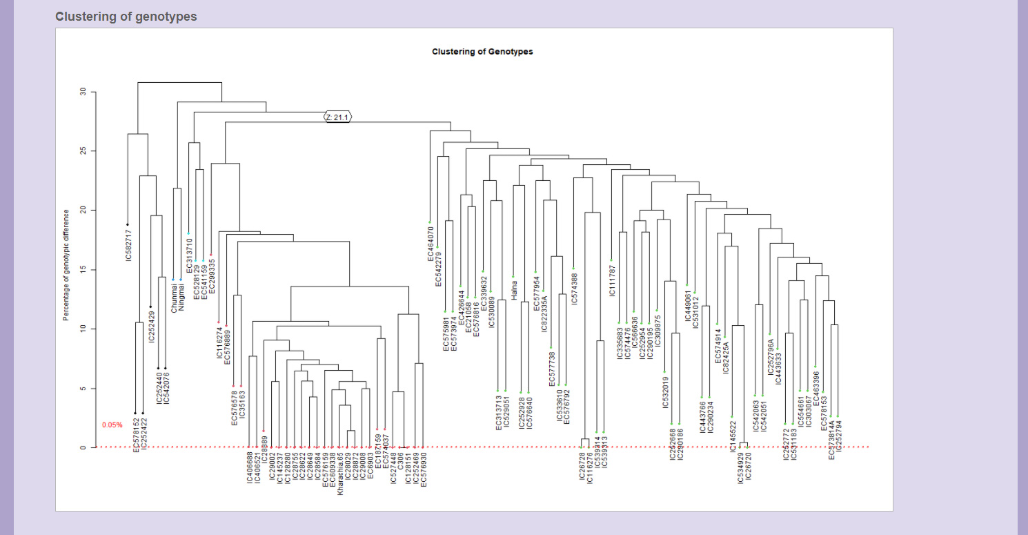
Genotype Clustering
In the genotype clustering, the genotypes are clustered based on the either total genotypic difference or homozygous difference. A dotted line for threshold is marked on the dendrogram below which the clusters represent duplicates. The clusters can be formed by selecting appropriate options for circular, rectangular or triangular clusters.

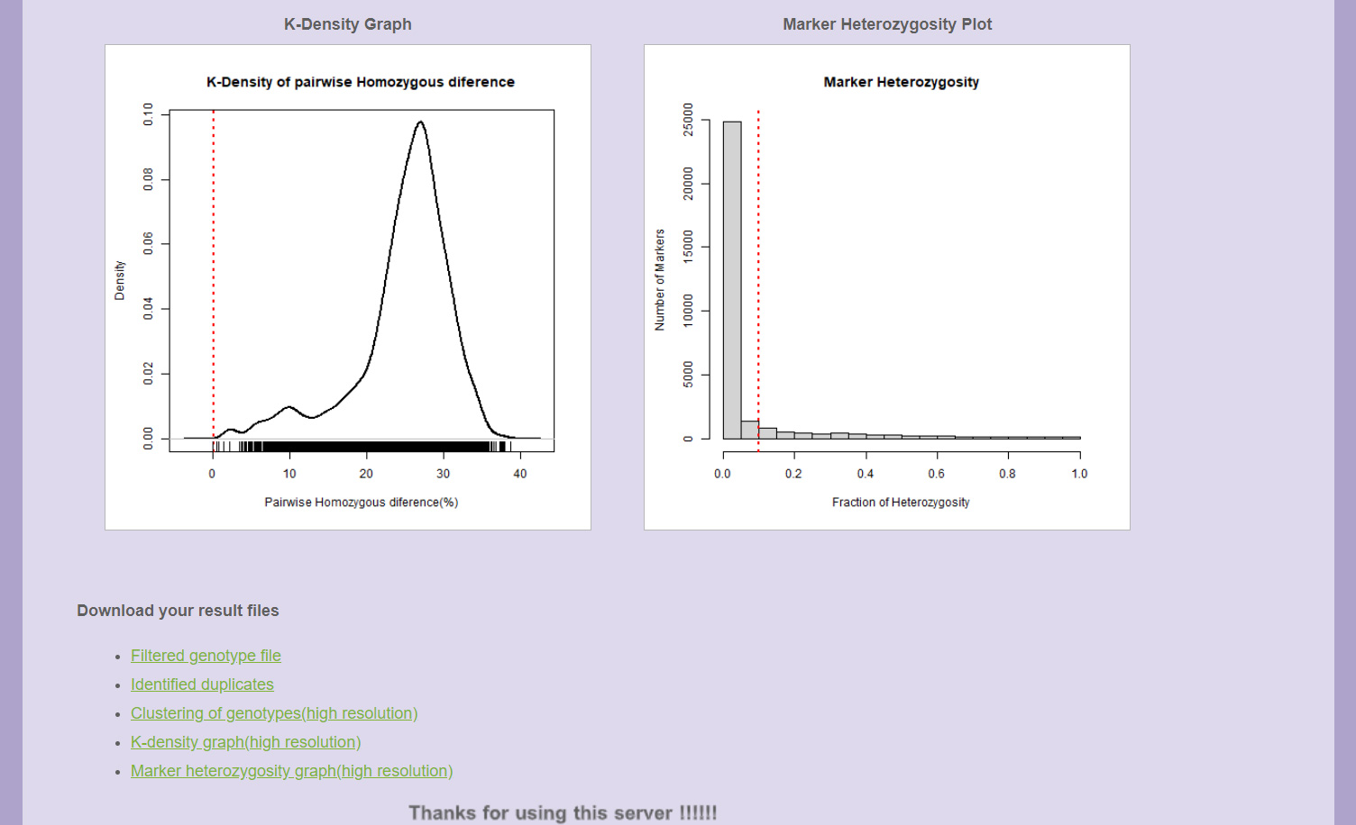
K-density graph
The K-density graph depicts the distribution of pairwise genotypic difference based on probability density function.

Marker heterozygosity plot
The marker heterozygosity plot gives an idea on the number of markers having the heterozygosity below the defined threshold.

Downloading the result files
The links for downloading the original figures, files along with the final processed genotype file in hapmap format is provided at the bottom of the result page.